Sequence level important requirements

To get the innovation id using user variable activity:



 To get the source file name when we pass the wild card pattern as source file to run the sequence:



To get the runtime and rundate in Sequence:





We can capture multiples variables in user variable activity:

Prallel Routine

How to create shared C code object and use them in datastage parallel routine?

Hello all, in this post i will give you information on datastage parallel routines and shared C code objects, and how can we create shared C code objects and use them in parallel routines.
Datastage Parallel Routine:
A parallel routine provides you feature to use external functionality written in C code to use in Datastage.
E.g.  Datastage does not provide regular expression functionality. So we can created shared object of regular expression functionality in C and used it in Datastage.
Steps:
1.       Create required function in C.

Here is a simple C function to add two numbers.
No need of Main.

#include
 
int sum_p(int a , int b)
{
c=a+b;
return c;
}

Suppose the name of above program is sum_pk.c

2.       Create shared object /library of the code.

Position Independent Object:
g++34 -fpic -c sum_pk.c

g++: GNU compiler available in Unix. g++34 is version of g++ available on our server.
-c : compiles code and creates object of file
-fpic: creates object with position independent code which is required for shared object/library

Object file with extension  .o will be created as sum_pk.o

a)      Shared Object:
Shared object is created from position independent object file created above.
g++34 -shared -o sum_pk.so  sum_pk.o

sum_pk.so is the shared object file created from sum_pk.o

b)      Shared library:
Shared library is also created from position independent object file created above.
g++34 -shared -o libsum_pk.so sum_pk.o

libsum_pk.so is the shared library file created from sum_pk.o

Shared library Vs Shared Object:

Shared Library	Shared object
A shared library file is linked to job at runtime and must be available at runtime.	A shared object file is linked to job at compile time.
Shared library name should start with “lib” and should have “.so” as extension E.g. libsum_pk.so	No such constraint on shared object.
Shared library should be present in predefined library paths. E.g. /opt/IBM/InformationServer/ASBNode/lib/cpp/ is the library path in our datastage installation	No such constraint on shared object.

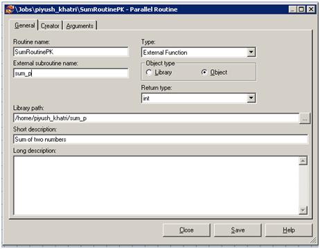
3.       Creating a parallel routine in Datastage:

• File>New>Routines>Parallel Routine
• Fill all the required values as:

Routine Name:  Any name with just alphanumeric characters only. No underscore as well.
External subroutine name: Name of the C function which we want to invoke
Type: External Function
Object Type: Library if you are using shared library or Object if you are using shared object.
Return Type: Return type of the C function
Library path: Library name with complete path
If shared library the path should be
                            /opt/IBM/InformationServer/ASBNode/lib/cpp/

Go to Arguments tab and enter details about the input arguments that the C function/ parallel routine will consume.
Save your routine to required folder.

Usage:

You need a transformer stage to use parallel routine external function in your job.
In Derivation pane of any port in transformer stage:
Right Click > DS_Routines> will call your riutine
E.g. SumRoutinePK(%a%, %b%)
Enter the required input parameters and it will return the required result.
sumRoutinePK(DSLink2.F1, DSLink2.F2)

String Functions in Transformer

1.  AlNum(%string%)

Allnum(“12345”) --- output-1

Allnum(“abcd”) --- output-1

Allnum(“ab125”) --- output-1

Allnum(“@a12345”) --- output-0

Allnum(“@a1 2345”) --- output-0

Except Special Symbols (Letters & Numbers) it will give output as “1”

2. Alpha(%string%)

Alpha (“abcd”) --- output-1

Alpha (“12345”) --- output-0

Alpha (“ab125”) --- output-0

Alpha (“@a12345”) --- output-0

Alpha (“@a1 2345”) --- output-0

3. Compactwhitespace(%string%)

     It reduces or replaces multiple spaces into single space.

Ex: CompactWhiteSpace("sud hee                  r") 

            Out Put: sud hee r

4. Space(length):

     Inserts no.of white spaces given in lengthy parameters.

        Ex:-Space(6):’Brahma’

       Output: Brahma

5 . Len(string):

Returns length of string in characters

     Ex:- Len(space(6):’Brahma’)

     Output---12

     Ex:- Len(“Brahma”)

      Output—6

6. Compare(String1,String2,[Justification]):       //case sensitive

      Compares String1 & String2,if String1 is greater than String2 it will result 1

            If String1 is less than String2,then it will result 1.

            If both the strings are equal then it will result 0.

            To compare String1 with String2, we give Justification:L

           To compare String2 with String1,we give Justification:R

     Ex:       Compare(“abcd”,”abc”,”L”)---output-1

                  Compare(“abcd”,”abc”,”R”)---output-0

                  Compare(“abc”,”Abc”)---output-1     Default Justification-L

                  Compare(“abc”,”abcd”)---output  -1

7. CompareNoCase(String1,String2):

             Same as Compare,but diff is this function is NOT case sensitive.

          In this function no argument called Justification.

8. CompareNum(String1,String2,length):

           Compares two strings up to the given length.

           Ex:-     CompareNum(“a”,”abc”,1)     output---0

                       CompareNum(“a”,”abcde”,5) output--    -1

           CompareNum(“abcde”,”a”,5) output---1

           CompareNum(“abcde”,”Abcde”,1)    output---1

           CompareNum(“Abcde”,”abcde”,1)    output--   -1

9. CompareNumNoCase(String1,String2,length):

          Same as CompareNum, diff is this function is NOT case sensitive.

          Ex:-     CompareNumNoCase(“Abcde”,”abcde”,5)   output---0

         CompareNumNoCase(“abxye”,”abcde”,5)    output---1

         CompareNumNoCase(“abcde”,”abxde”,5)    output--  -1

10. Upcase(String):

           Change all lowercase letters in a string to uppercase.

           Ex:-     Upcase(“brahma”)       output—BRAHMA

           Upcase(“braHma”)      output----BRAHMA

11. DQuote(String):

          Enclose a string in double quotation marks.

         Ex:-     DQuote(Upcase(“brahma”))   output---“BRAHMA”

        DQuote(‘brahma’)                  output---“brahma”

12. Field(String,delimiter,occurrence,number):

          Returns the substring before delimiter based on occurrence we are given.

            Ex:-     Field(“br_ah_ma_na”,”_”,2)   output---ah

         Here ah is substring before the second occurrence of delimiter ‘_’.

Field(“br_ah_ma_na”,”_”,3)   output---ma

         Here after ma _ is third occurrence.

Field(“br_ah_ma_na”,”_”,1,4)            output---br_ah_ma_na

Field(“br_ah_ma_na”,”_”,1,2)            output---br_ah

Field(“br_ah_ma_na”,”_”,1,3)            output---br_ah_ma

Field(“br_ah_ma_na_a”,”_”,1,5)        output---br_ah_ma_na_a

 Note:-

          Field(“brahmananda”,”a”,2)   output—hm

   Here ‘a’ is delimiter

         Field(“brbhmananda”,”a”,2)   output—n

         Field(“brhhmananda”,”a”,1)   output—brhhm

          Field(“brahmananda”,”a”,1,3)  output—brahman

13. Index(String,substring,occurrence):

        Returns starting character position of substring.

        Ex:-     Index(“brahma”,”a”,1)            output---3

        Index(“brahma”,”a”,2)            output---6

        Index(“brahmananda”,”a”,3)  output---8

        Index(“brahmananda”,”na”,1)  output---7

14. Convert(fromlist,tolist,Expression)

      Converts specified character in a string(given in expression arg) to designated replacement character

      Ex:-  convert(“a”,”y”,”brahma”)

   o/p:byhmy

             convert(“ah”,”y”,”brahma”)

   o/p:brymy

      This function performs character replacement, but not word.

      Ex:  convert(“brahma”,”msrmad”,”brahma”)

15. Count(String,Substring):

      Count number of times a Substring occurs in a String.

      Ex:Count(“brahma”,”a”)

            o/p:2

           Count(“brahmabaabaaba”,”ab”)

            o/p:3

          Count(“brahmabaabaaba”,”ba”)

            o/p:3

16. DCount(String,Delimiter):

      Count number of delimited fields in a string.

     Ex:  DCount(“br-ah-ma-na”,”_”)-------o/p:4

             DCount(“br,ah,ma,na”,”,”)-------o/p:5

             DCount(“br,ah-ma,na”,”,”)-------o/p:4

    ah-ma, treats as one field

17. Downcase(String):

       Change all uppercase letters in a String to lowercase

     Ex:  Downcase(“BRAHMA”)------o/p:brahma

             Downcase(“brHMA”)------o/p:brahma

             Downcase(“BRAhma”)------o/p:brahma

18. Left(String,length)

        Returns leftmost ‘n’ characters of the string, where n is length.

      

       Ex:  Left(“brahmananda”,4) o/p:brah

               Left(“bra__hmananda”,6) o/p:bra_hm

19. Right(String,Length)

      Returns rightmost ‘n’ characters of the string

    

      Ex:   Right(“brahmananda”,4) o/p:anda

20. Num(String)

     Returns 1 if string can be converted to a number.

     

     Ex:    Num(“brah”)    o/p=0

              Num(“369”)     o/p=1

21. PadString(String,PadString,Padlength)

       Returns the string padded with the optional pad character and padlength is the number of times it add to the original string

    

      Ex:    PadString(“brahma”,”+”,5)    o/p:brahma+++++

                PadString(“brahma”,”reddy”,5)   o/p:brahmarrrrr

22. Str(String,repeats)

       Repeats the input string no.of times given in repeats

    

      Ex:  Str(“mbnr”,2)    o/pmbnrmbnr

23. StripWhiteSpace(String)

       Returns the string after stripping (removing) all white space from it.

     

     Ex:  StripWhiteSpace(“br a h ma”)   o/p:brahma

Steps to be followed for implementing SCD II

Read the incoming records through any input stage like sequential file/dataset/table.

• Do the required processing for the incoming data.

• After the above processing step, pass the data into the change capture stage.

• The change capture should be having two input links- one is the before dataset and the other is the after dataset. For our job, the before dataset should be the active records present in the table. The active records are all those records which are having EXPR_DT=’2999-12-31’. The after dataset will be the incoming data passed into change capture after all the necessary processing.

• The change capture stage compared the before dataset and after dataset and produces 4 change_codes for each of the records. The 4 change codes are as follows:

“0” – Copy code (The code indicates the after record is a copy of the before record)

“1”-Insert code (The code indicates a new record has been inserted in the after set that did not exist in the before set.)

“2”-Delete code(The code indicates that a record in the before set has been deleted from the after set)

“3”-Edit code(the code indicates the after record is an edited version of the before record)

The copy records are not passed in the change captured stage as since we need only edited, insert records fro SCD II implementation.

• Use a filter stage to separate the records that needs to be expired and inserted.

• Filter the records with change_code = “1 or 3” into the insert records link. Filter the records with change_code=” 3” into update/expiry link.

• The records with change_code=3 are edited records. So the original records corresponding to these edited records are to be made in-active (expired). We can make the records inactive by changing the EXPR_DT<> ‘2999-12-31’.So to make the record inactive change the EXPR_DT with a valid date. For e.g. you can use make the EXPR_DT as the date one less than the date on which you are loading the data into the table. We will assume that we are loading the data on 2008-08-15.So the EXPR_DT for inactive records would become ‘2008-08-14’. The date 2008-08-15 can be made as the EFCT_DT for records to be inserted.

• To get the original records which needs to be expired, “look-up” the target table for all the records with change_code=3 which are filtered out separately. Get the original record along with the EFCT_DT of the original record. Then update the records EXPR_DT to ‘2008-08-14’ in the table. Now the original records are made inactive (expired).

• The new updated record (change_code=3) needs to be in table along with the new insert records(change_code=1).This data is filtered out from the “filter” stage and inserted into the table with EFCT_DT=”Data of loading” i.e. “2008-08-15” and EXPR_DT=”2999-12-31” 





 ---------------------------------

Datastage Implementations – Slowly Changing Dimensions

Basics of SCD

Slowly Changing Dimensions (SCDs) are dimensions that have data that changes slowly, rather than changing on a time-based, regular schedule.

Type 1

The Type 1 methodology overwrites old data with new data, and therefore does not track historical data at all.

Here is an example of a database table that keeps supplier information:

-------------------------------------------------------------------

Supplier_Key

Supplier_Code

Supplier_Name

Supplier_State

123

ABC

Acme Supply Co

CA

--------------------------------------------------------------------

In this example, Supplier_Code is the natural key and Supplier_Key is a surrogate key. Technically, the surrogate key is not necessary, since the table will be unique by the natural key (Supplier_Code). However, the joins will perform better on an integer than on a character string.

Now imagine that this supplier moves their headquarters to Illinois. The updated table would simply overwrite this record:

----------------------------------------------------------------

Supplier_Key	Supplier_Code	Supplier_Name	Supplier_State
123	ABC	Acme Supply Co	IL

---------------------------------------------------------------

Type 2

The Type 2 method tracks historical data by creating multiple records for a given natural key in the dimensional tables with separate surrogate keys and/or different version numbers. With Type 2, we have unlimited history preservation as a new record is inserted each time a change is made.

In the same example, if the supplier moves to Illinois, the table could look like this, with incremented version numbers to indicate the sequence of changes:

-----------------------------------------------------------------

Supplier_Key	Supplier_Code	Supplier_Name	Supplier_State	Version
123	ABC	Acme Supply Co	CA	0
124	ABC	Acme Supply Co	IL	1

-----------------------------------------------------------------

Another popular method for tuple versioning is to add effective date columns.
-----------------------------------------------------------------------------------

Supplier_Key	Supplier_Code	Supplier_Name	Supplier_State	Start_Date	End_Date
123	ABC	Acme Supply Co	CA	01-Jan-2000	21-Dec-2004
124	ABC	Acme Supply Co	IL	22-Dec-2004

------------------------------------------------------------------------------------

The null End_Date in row two indicates the current tuple version. In some cases, a standardized surrogate high date (e.g. 9999-12-31) may be used as an end date, so that the field can be included in an index, and so that null-value substitution is not required when querying.

How to Implement SCD using DataStage 8.1 –SCD stage?

Step 1: Create a datastage job with the below structure-

1. Source file that comes from the OLTP sources
2. Old dimesion refernce table link
3. The SCD stage
4. Target Fact Table
5. Dimesion Update/Insert link 
   
   

   Figure 1

Step 2:  To set up the SCD properties in the SCD stage ,open the stage and access the Fast Path

Figure 2

Step 3: The tab 2 of SCD stage is used specify the purpose of each of the pulled keys from the referenced dimension tables.

Figure 3

Step 4: Tab 3 is used to provide the seqence generator file/table name which is used to generate the new surrogate keys for the new or latest dimesion records.These are keys which also get passed to the fact tables for direct load.

Figure 4

Step 5:  The Tab 4 is used to set the properties for configuring the data population logic for the new and old dimension rows. The type of activies that we can configure as a part of this tab are:

1. Generation the new Surrogate key values to be passed to the dimension and fact table
2. Mapping the source columns with the source column
3. Setting up of the expired values for the old rows
4. Defining the values to mark the current active rows out of multiple type rows

Figure 5

Step 6: Set the derivation logic for the fact as a part of the last tab.

Figure 6

Step 7: Complete the remaining set up, run the job

Debug in Datastage 8.7

Step 1 : Right click on the link where you want to create a break point       

  Step 2 : Then click on Toggle Breakpoint                                                          

Step 4 :  Then From the Menu bar click "Debug" then click "Go".

Then Job Run window and Debug window will appear, then provide required parameter values and click ok on Jon Run window.

It will show like below when Debug is running

Next it will show up the first row values like below.We can change number of rows you want to see by clicking "Edit Break Point" from the "Menu > Debug " or by right clicking on the "Break Point" that we created in Step 1.

Data Stage Sequential File Stages (Import and Export) Performance Tuning

Improving Sequential File Performance

If the source file is fixed/de-limited, the Readers Per Nodeoption can be used to read a single input file in parallel at evenly-spaced offsets. Note that in this manner, input row order is not maintained.
 If the input sequential file cannot be read in parallel, performance can still be improved by separating the file I/O from the column parsing operation. To accomplish this, define a single large string column for the non-parallel Sequential File read, and then pass this to a Column Import stage to parse the file in parallel. The formatting and column properties of the Column Import stage match those of the Sequential File stage.
On heavily-loaded file servers or some RAID/SAN array configurations, the environment variables $APT_IMPORT_BUFFER_SIZEand $APT_EXPORT_BUFFER_SIZEcan be used to improve I/O performance. These settings specify the size of the read (import) and write (export) buffer size in Kbytes, with a default of 128 (128K). Increasing this may improve performance.
Finally, in some disk array configurations, setting the environment variable $APT_CONSISTENT_BUFFERIO_SIZEto a value equal to the read/write size in bytes can significantly improve performance of Sequential File operations.

Partitioning Sequential File Reads

Care must be taken to choose the appropriate partitioning method from a Sequential File read:
Don’t read from Sequential File using SAME partitioning! Unless more than one source file is specified, SAME will read the entire file into a single partition, making the entire downstream flow run sequentially (unless it is later repartitioned).
When multiple files are read by a single Sequential File stage (using multiple files, or by using a File Pattern), each file’s data is read into a separate partition. It is important to use ROUND-ROBIN partitioning (or other partitioning appropriate to downstream components) to evenly distribute the data in the flow.

Sequential File (Export) Buffering

By default, the Sequential File (export operator) stage buffers its writes to optimize performance. When a job completes successfully, the buffers are always flushed to disk. The environment variable $APT_EXPORT_FLUSH_COUNTallows the job developer to specify how frequently (in number of rows) that the Sequential File stage flushes its internal buffer on writes. Setting this value to a low number (such as 1) is useful for realtime applications, but there is a small performance penalty associated with increased I/O.

 Reading from and Writing to Fixed-Length Files

Particular attention must be taken when processing fixed-length fields using the Sequential File stage:
If the incoming columns are variable-length data types (eg. Integer, Decimal, Varchar), the field width column property must be set to match the fixed-width of the input column. Double-click on the column number in the grid dialog to set this column property.

If a field is nullable, you must define the null field value and length in the Nullable section of the column property. Double-click on the column number in the grid dialog to set these properties.

When writing fixed-length files from variable-length fields (eg. Integer, Decimal, Varchar), the field width and pad string column properties must be set to match the fixed-width of the output column. Double-click on the column number in the grid dialog to set this column property.
 To display each field value, use the print_field import property. All import and export properties are listed in chapter 25, Import/Export Properties of the Orchestrate 7.0 Operators Reference.

 Reading Bounded-Length VARCHAR Columns

Care must be taken when reading delimited, bounded-length Varchar columns (Varchars with the length option set). By default, if the source file has fields with values longer than the maximum Varchar length, these extra characters will be silently truncated.
Starting with v7.01 the environment variable
$APT_IMPORT_REJECT_STRING_FIELD_OVERRUNS will direct DataStage to reject records with strings longer than their declared maximum column length.

Environmental variables in Datastage

Basically Environment variable is predefined variable those we can use while creating DS job.we create/declare these variables in DS Administrator.while designing the job we set the properties for these variables.For Example Database Uname/Pwd we declare these variables in Admin and set the values Scott and Tiger values in the properties tab in the Menu(Parameters tab)